Training Transformers: A Review
It has been a while since I’ve trained models from scratch, but now that I am revisiting AI I wanted to work on a nice little exercise to recalibrate my intuition on training neural networks. And since transformers seems to be used everywhere these days, I figured I’d try to implement a mini GPT-2 model.
I imagine this website will be somewhat of a living document that I’ll update as I learn more, not just on ML but also on tech required to usher in the age of abundance. Expect more educational(for myself) posts like this from me in the future as I learn stuff to build my projects.
This post and an upcoming post in particular contains my notes and learnings about language models from and beyond the original Transformer paper (Vaswani et al 2017) and its variants.
Note: The posts are mostly intended to be a helpful note for myself. I deliberately avoided looking at other implementations to challenge myself and learn more through trial and error. I won’t include all details from the transformer or the gpt papers, only mentioning details when they actually matter. While I hope this serves as a helpful note, please let me know if I’ve missed or misunderstood any important details via X.
Overview
In this post, I’ll try to train a mini GPT-2 model, which is just a scaled up decoder only transformer with a single GPU. I’ll cover the following:
-
Describe my data and tokenization approach
-
Go over my intuition behind attention mechanisms with examples
-
Explain how positional encoding fits in so the model knows token order
-
Discuss regularization implementation details (dropout, layernorm, residual connections)
-
Talk about training issues I encountered and respective solutions
Data and Tokenization
I first quickly trained a small proof-of-concept using a toy dataset of short phrases like “car drives on”, “phones connect people”, etc. This led to some interesting problems.
With this dataset the model produced a degenerate attention pattern and a trivial solution where each token only attended to itself(one hot vector attention vectors for each tokens). Foolishly enough I tried debugging the model until I realized the implementation wasn’t the issue; the problem was simply a (major)lack of data.
So then I downloaded the C4 from the dataset repo, and given that I’m training a mini LLM selected only the first 300,000 sentences. I then tried these two tokenizers
Tokenization Approaches
I first experimented with a custom word-based tokenizer:
1. Custom Word-Based Tokenizer
This simple approach:
-
Counted word frequencies in the dataset
-
Selected top 50k most frequent words as vocabulary
-
Mapped everything else to
<unk>
This actually ended up in a decent model that learnt syntax and grammar pretty well. However, it
predicted too many <unk> tokens for any word not in the top 50k, which were quite a lot(there were
around 160k unique vocab in the dataset). The model would keep generating things like ‘This is a
nice <unk>’, ‘Lets go to the <unk>’ ,etc.
2. BPE Tokenizer
To fix this, I switched to Byte-Pair Encoding (BPE). I trained it on my corpus (a subset of C4). For about 300k sentence samples and 50k vocab size, BPE ended up producing ~143M tokens total. BPE works by merging the most frequent character pairs, creating subword units so that it drastically reduce unrecognizable tokens. So by training a BPE on my data, the model gets a tokenizer better aligned with the text the model is learning from.
def train_bpe_tokenizer(sentences, vocab_size=50000):
    """Train a BPE tokenizer on the given sentences"""
    tokenizer = Tokenizer(BPE(unk_token="<unk>"))
    trainer = BpeTrainer(
        vocab_size=vocab_size,
        special_tokens=["<pad>", "<unk>", "<s>", "</s>"],
    )
    tokenizer.pre_tokenizer = Whitespace()

    # Train the tokenizer
    tokenizer.train_from_iterator(sentences, trainer)
    return tokenizer
I also tried the tiktoken gpt2 tokenizer, which was trained on a different corpus. Using a mismatched tokenizer produced weird partial decodes so the model wasn’t learning properly.
In the final training scripts, I mostly rely on this BPE tokenizer. Whenever the model sees a sentence, it breaks it into subwords, maps them to IDs, and any truly unknown text can be spelled out via partial merges.
Attention Folks
There are probably much better explanation of attention mechanism elsewhere (i.e ask chatGPT) but I’m going to try my best here.
At a high level, attention lets each token communicate with every other token in the sequence to gather context.
Think of a sentence: “Car drives on”. If I want to predict the next token (“roads,” for example), the word “on” needs to figure out what it’s referencing. “On” by itself is ambiguous - it could mean “turned on,” “switched on,” “located on,” etc. But with attention, the token “on” can look back at “car” and “drives” to gather that the context is about a car driving, so the next token is likely “roads,” or something similar. Pretty simple concept, but the question is how to know exactly where to look?
I’ll start by laying out a very simplified attention mechanism implementation where I explain each part below.
# Part A. x is the input of shape (B,S) where B is the number of batches, S is the sequence length(number of tokens) of each batch.
# You get the query, key, and value vector for each token for each batch, which results in a
# Q, K, (B, S, embed_dim) matrix.
# w_q, w_k, w_v are all learnable weights
Q = w_q(x)
K = w_k(x)
V = w_v(x)

# Compute the attention scores for each token with Q dot K.T
d_k = Q.size(-1)
attention_scores = torch.matmul(Q, K.transpose(-2, -1)) / math.sqrt(d_k)  # (B, S, S)

# Part B. the causal mask to zero out attention scores future tokens
# for each token, you ignore the attention scores of tokens in front
mask = ~torch.triu(torch.ones(S,S), diagonal=1).bool().unsqueeze(0).unsqueeze(0).to(x.device)
scores = attention_scores.masked_fill(mask == 0, float('-inf'))

# Part C. this makes the attention scores sum to one for every token
attn_weights = torch.softmax(attention_scores, dim=-1)  # (B, nH, S, S)

# the resulting output is, for each token vector, a new token vector that encapsulates the context
output = torch.matmul(attn_weights, V)        # (B, nH, S, head_dim)

# this output then just goes through a linear layer to predict the next token logits
Part A. Each token’s embedding can be used to create a query and a key vector. For a given token, the query asks: “Among these other tokens in the sequence, whose information do I need?”, after which the keys of other tokens answer, “I have certain context you need”. This is done by obtaining the “similarity score” between the query and the key, which is why the dot product computation of q and k vectors comes in.
Think of it like a smart search engine:
-
Query (q) = “What you’re looking for”
-
Key (k) = “Labels/tags describing each piece of content”
-
The more similar q and k are, the more relevant that content is(need to attend to)
For the given words “Car drives on”, the “similarity scores” of each words in the sentence between itself and every word(including itself) needs to be computed, which would result in a 3x3 matrix called the attention matrix.
For the sentence “Car drives on”, an example attention matrix might look like:
\[\begin{bmatrix} 1.0 & 0.0 & 0.0 \\ 0.5 & 0.5 & 0.0 \\ 0.4 & 0.4 & 0.2 \end{bmatrix}\]Each row represents similarity scores of a token with every other token in the sequence including itself. The first row consists of the similarity scores of the word ‘Car’ between the words ‘Car’, ‘drives’, ‘on’ and the second row consists of the similarity scores of the word ‘drives’ for ‘Car’, ‘drives’, ‘on’, and lastly similarly for the ‘on’ token for the third row.
This score matrix is obtained by taking the dot product of all the query and key vectors, which is then scaled by the dimensionality of the Q(or K, its the same) matrix so that the subsequent softmax doesn’t blow stuff up,
\[\text{AttentionMatrix}(Q, K) = \frac{QK^T}{\sqrt{d_k}}\] \[\begin{align*} where \\ Q &= \text{query matrix} \\ K &= \text{key matrix} \\ d_k &= \text{dimension of key/query vectors} \end{align*}\]Part B. Also, in a decoder-only model like GPT-2, each token can only attend to the tokens before it (using the causal mask). Effectively, this exists so that the model can practice predicting the future based on the past, without peaking into the future. So a mask is applied to the attention matrix so that when multiplied with the V matrix it will zero out all future tokens(no words will attend to its future words).
In the example 3x3 above, a causal mask is already applied. The first word Car only attends to itself, while the second word drives attends to Car and itself, and the third word on attends to Car, drives and itself.
Part C. Softmax is applied to the attention scores so that they are normalized. After which, it needs to be multiplied by the actual token embeddings (the \(V\) matrix which consists of embedding vectors \(v\) for all tokens), so that each [word vector] \(v_i\) updates itself to [some new vector] \(v_i'\) that encapsulates the context of the sequence. When updating to \(v_i'\), the attention scores dictate how much each of the past tokens in that sequence needs to be attended to.
\[\text{Attention weighted output}(Q, K, V) = \text{softmax}\left(\frac{QK^T}{\sqrt{d_k}}\right)V\] \[= \begin{bmatrix} v_1' \\ v_2' \\ v_3' \end{bmatrix} = \begin{bmatrix} 1.0v_1 + 0.0v_2 + 0.0v_3 \\ 0.5v_1 + 0.5v_2 + 0.0v_3 \\ 0.4v_1 + 0.4v_2 + 0.2v_3 \end{bmatrix} = V'\]For example, in the case of the token ‘on’, that [some new ‘on’ vector] would be a linear combination of ‘Car’, ‘drives’ and ‘on’ embedding vectors, such that the final ‘on’ vector would encapsulate the entire context and be much better equipped to predict the next token ‘road’.
This \(V'\) is then passed through a feedforward layer to predict the next token logits.
Parallelism: The beauty of attention is that, even though we do next-token prediction based on all previous context, which intuitively should be a recursive process, at training time the model can process the entire sequence in parallel. This is more efficient than recurrent models (RNNs) that process one token at a time one at a time, making it hard to parallelize and thus train them at scale.
Multi-Headed Attention
Although omitted in the code example above, sufficiently large transformers are trained by splitting the embedding dimension into multiple heads. This is motivated by the fact that a single attention mechanism may struggle to capture different types of relationships between tokens simultaneously. For example, a token might need to attend to both syntactic dependencies (like subject-verb agreement) and semantic relationships (like topic relevance) at the same time. By having multiple attention heads that operate in parallel on different projections of the input, the model can learn to specialize different heads for different aspects of the relationships between tokens.
This simply adds another batch operation to the mat muls above. We then concatenate the heads’ outputs into one representation before passing it through a final linear layer.
Positional Encoding
Transformers are permutation-invariant if we just do attention alone. That means the set of tokens [car, drives, on] is the same as [drives, car, on] to the raw attention mechanism unless we inject positional information.
Positional encoding is how we do this, where for each token vector, we add position information vectors to the token embeddings, before passing it through the attention mechanism. A common technique is the sinusoidal approach. Now the model can distinguish “car drives on” from “drives car on,” ensuring “on” knows how to make sense of the context.
In the gpt-2 paper, the author states that separate learnable weights are used for this encoding vectors but for simplicity I just used the sinusoidal implementation.
How tokens are predicted
To summarize the entire process for a sequence x going through a transformer layer to predict the next tokens:
\[\begin{align*} \text{Step 1: Embedding} &: x \rightarrow X = \text{Embedding}(x) + \text{PositionalEncoding}(x) \\ &\text{where } x \text{ is input sequence of length } L \\ &X \text{ is matrix of size } L \times d_{emb} \end{align*}\] \[\begin{align*} \text{Step 2: Attention} &: X \rightarrow V' = \text{softmax}\left(\frac{QK^T}{\sqrt{d_k}}\right)V \\ &\text{where } Q,K,V \text{ are linear projections of } X \end{align*}\] \[\begin{align*} \text{Step 3: FFN} &: V' \rightarrow V'' = W_2(\text{GeLU}(W_1V' + b_1)) + b_2 \end{align*}\] \[\begin{align*} \text{Step 4: Logits} &: V'' \rightarrow W_{out}V'' + b_{out} \\ &\text{output shape: } L \times V_{size} \text{ (vocab size)} \end{align*}\] \[\begin{align*} \text{Step 5: Sample} &: \text{logits} \rightarrow \text{predictions} = \text{multinomial}(\text{softmax}(\text{logits})) \\ &\text{output shape: } L \text{ (sequence of token indices)} \end{align*}\]Where the attention matrix is masked to be lower triangular (causal masking), and each step preserves the sequence length L while transforming the embedding dimensions.
You can see that L length goes in, L length comes out. For example, if input sequence length is L=3 like “This road is”, the output logits will also have length L=3, predicting the next token for each position: “road is blocked”.
There is model code in the colab notebook, its quite simple(only ~100 lines)
Regularization Techniques
Regularization is in general important for stabilizing training and preventing overfitting. In Transformers, we typically use:
-
Dropout: I applied dropout to attention weights and feed-forward sub-layers. This randomly zeroes out a fraction of values to reduce over-dependence on particular neurons.
-
Residual Connections: Each sub-layer does x = x + sublayer_output, letting the model preserve the original embedding while layering on transformations. This helps gradient flow and prevents vanishing or exploding gradients.
-
LayerNorm: Normalizes each token’s embedding vector to have stable mean/variance. Typically used before or after each attention/feed-forward sub-layer, e.g., pre-norm or post-norm.
These definitely helped stabilize the validation loss, though the effect was less dramatic compared to simply increasing data size and model capacity.
Pre-Norm vs. Post-Norm
A side note: The original attention paper applied layer norm after the attention layer, while GPT-2 typically does pre-norm(apply before attention). Some also add a final layernorm after the last layer, as did I in my implementation.
Training Issues I ran into and Solutions
- Degenerate Attention Matrices
When I worked with tiny datasets, sometimes each token just attended to itself or the first token in the sequence(one-hot vectors). That’s a valid “shortcut” solution if the task is trivial, but wasn’t able to generalize to unseen data at all(there was a huge training and validation loss discrepancy).
Solution: I simply added more data (C4 subset of 300k samples, ~150M tokens after BPE). This forced the model to learn more generalizable relationships.
- Exploding Loss
Occasionally, the training loss would blow up after a few hundred epochs.
Solution: Again, this only happened when the dataset was tiny. Both gradient clipping and a better learning-rate scheduling did not help until I simply added more data.
- Slow or Minimal Loss Convergence
Solution: I found increasing context length from 8 to 50 ~ 100 significantly improved loss convergence. Quite intuitive since the network sees more information for prediction.
Conclusion
Overall, it was quite refreshing to observe the scaling laws manifest itself quite clearly in practice - even at tiny scales like this. More data and compute consistently led to better results, even at this small scale.
I got the jist of the implementation in a few hours but I coudn’t quite get the model to work besides predicting some basic grammar structures. Only after I stopped obsessing over understanding and debugging neural network training dynamics, and instead focused on scaling up the model size and dataset, did everything kind of fixed itself.
Also note that this is just pretraining, not chatgpt. The pretraining phase is where most of the heavy lifting is done, and it’s the step most tutorials teach you about when you’re learning about language models in a pedagogical setting. But to make this into a production grade chatbot theres a whole lot more to do.
In that regard, some key topics I haven’t covered: post-training techniques (RLHF, instruction tuning), mixed precision training, hardware optimizations, and KV caching for efficient inference.
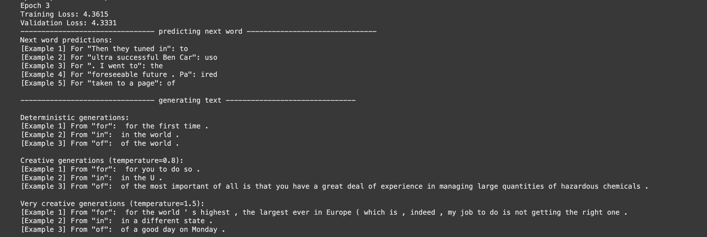
You can check out my implementation in this google colab notebook. You can just run it if you have a GPU. I had the pro version so I ran it with A100, but had to cut it off after 7 hours, so the model is not fully trained. But here are some of the results.