Quantum Computing 1: Deutsch-Jozsa Algorithm

13 Mar 2025

I recently started learning quantum computing techniques and the Deutsch-Jozsa Algorithm applied to the Bernstein-Vazirani problem was the first algorithm I encountered that I can see actually being potentially useful(at least for its variants). This post will not cover the vanilla Deutsch’s algorithm.

The Deutsch-Jozsa algorithm belongs to a class of algorithms called quantum query algorithms that serves to determine the properties of a function without any prior knowledge of the function’s properties or parameters. The algorithm is given a black box function \(f: \{0,1\}^n \rightarrow \{0,1\}\) that maps a set of inputs \(x\) to a set of outputs \(y\). When running the algorithm, the computer can only ‘query’ \(f\), observe how \(x\) relates to \(y\), and infer the properties or parameters of \(f\).

From this description, an immediate intuitive solution is to try a lot of possible inputs, observe the output, and then infer what \(f\) is. For some cases, this brute force approach happens to be the optimal solution. So can quantum algorithms speed this search significantly?

A related and useful thought experiment is the Bernstein-Vazirani problem. Here a function \(f\) is defined as a (binary) linear function of the input \(x\), and there exists a binary vector \(s = (s_{n-1} \cdots s_0)\) for which \(f(x) = s \cdot x\) for all \(x \in \Sigma^n\), where

\[x \cdot s = \begin{cases} 1 & \text{if } x_{n-1}s_{n-1} + \cdots + x_0s_0 \text{ is odd} \\ 0 & \text{if } x_{n-1}s_{n-1} + \cdots + x_0s_0 \text{ is even} \end{cases}\]

The problem, or the algorithm’s objective, is to determine the binary vector \(s\) given query access to \(f\). We obviously want to query \(f\) as few times as possible.

Classical Solution

With classical computing, the most optimal solution is quite trivial. You simply evaluate the function \(n\) times with different one-hot vectors each iteration

\[f(1000\ldots0) = s_0\] \[f(0100\ldots0) = s_1\] \[f(0010\ldots0) = s_2\] \[\vdots\] \[f(0000\ldots1) = s_{n-1}\]

since \((1,0,0,\ldots,0) \cdot (s_0, s_1, \ldots, s_{n-1}) = s_0\) and so forth. Note that this requires \(n\) queries of \(f\) to determine the secret vector \(s\).

Quantum Solution

The Deutsch-Jozsa algorithm can however solve this problem in a single query.

Intuitively, the algorithm constructs a superposition of all possible solutions of \(s\) and then queries the function \(f\) in parallel(with quantum mechanics!) across all possible \(s\) to verify the parameters of \(s\).

This is an example of a quantum circuit that solves the Bernstein-Vazirani problem, with 4 qubits and 1 ancilla qubit. Each x qubits represent possible solutions of \(s\), where the circuit can ‘test’ all possible solutions in parallel. The y is called the ancilla qubit, and it is present for the sole purpose of making the oracle function work as a unitary operation(by storing the output of the function).

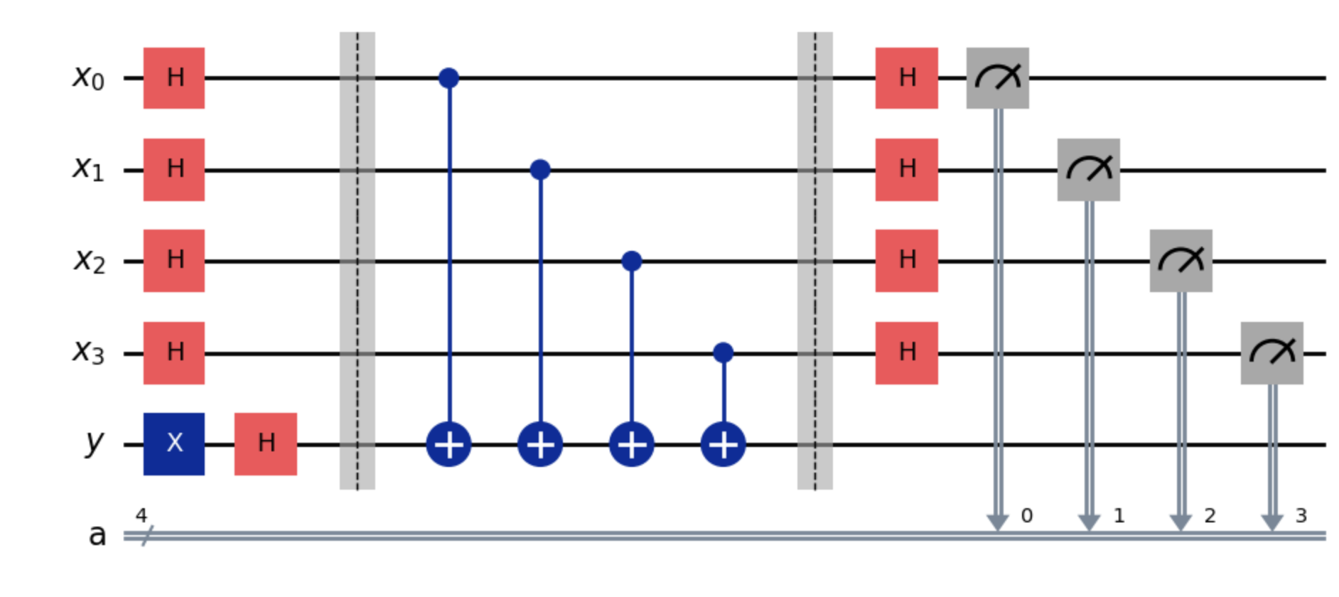The circuit is composed of 4 steps: 1. Hadamard 2. Oracle 3. Hadamard 4. Measure

0. Define inputs

Let’s define our quantum system with \(n+1\) qubits: \(n\) qubits for the input register \(|x\rangle\), where \(x \in \{0,1\}^n\) and \(1\) ancilla qubit \(|y\rangle\) for storing the function output. (Look up Deutsch algorithm for more details on this technique) x and y are standard basis states, with \(|0\rangle\) for the input register and \(|1\rangle\) for the ancilla qubit.

1. Apply Hadamard gates to the input register

We then apply \(n\) Hadamard gates to the input register to create a superposition of all possible inputs. A general Hadamard gate on a qubit \(|x\rangle\) formed with \(n\) qubits can be represented as:

\[H^{\otimes n} |x\rangle = \frac{1}{2^{n/2}} \sum_{y \in \Sigma^n} (-1)^{x \cdot y} |y\rangle\]

Turning to our example, after the first layer of Hadamard gates is performed, the state of the \(n+1\) qubits is

\[\left|{-}\right\rangle \otimes \frac{1}{2^{n/2}} \sum_{x \in \Sigma^n} \left|{x}\right\rangle\]

2. Query the oracle

Now we query the oracle, which applies the function \(f(x) = s \cdot x\) to our superposition state. The oracle transforms the state as follows(using phase kickback):

\[\left|{-}\right\rangle \otimes \frac{1}{2^{n/2}} \sum_{x \in \Sigma^n} \left|{x}\right\rangle \rightarrow \left|{-}\right\rangle \otimes \frac{1}{2^{n/2}} \sum_{x \in \Sigma^n} (-1)^{f(x)} \left|{x}\right\rangle\]

3. Apply Hadamard again to oracle output

Next we want to collapse the superposition on x after the oracle query using Hadamard again. Applying the same generalized Hadamard solution from 1 to 2,

\[\left|{-}\right\rangle \otimes \frac{1}{2^{n}} \sum_{x \in \Sigma^n} \sum_{y \in \Sigma^n} (-1)^{f(x)+x \cdot y} \left|{y}\right\rangle\]

Using the formula for the action of the second layer of Hadamard gates, we can simplify our state. Since we’re promised that \(f(x) = s \cdot x\) for some secret string \(s\), we can rewrite the state as:

\[\left|{-}\right\rangle \otimes \frac{1}{2^{n}} \sum_{x \in \Sigma^n} \sum_{y \in \Sigma^n} (-1)^{s \cdot x + x \cdot y} \left|{y}\right\rangle\]

Since we’re working with binary values in the exponent of \((-1)\), we can replace addition with XOR (\(\oplus\)), as all that matters is whether the exponent is even or odd:

\[\left|{-}\right\rangle \otimes \frac{1}{2^{n}} \sum_{x \in \Sigma^n} \sum_{y \in \Sigma^n} (-1)^{(s \cdot x) \oplus (x \cdot y)} \left|{y}\right\rangle\]

We can use the identity \((s \cdot x) \oplus (y \cdot x) = (s \oplus y) \cdot x\), which can be derived by expanding the dot products and applying the bit-level identity \((ac) \oplus (bc) = (a \oplus b)c\). This gives us:

\[\left|{-}\right\rangle \otimes \frac{1}{2^{n}} \sum_{x \in \Sigma^n} \sum_{y \in \Sigma^n} (-1)^{(s \oplus y) \cdot x} \left|{y}\right\rangle\]

Now we can apply another important identity: for any binary string \(z\),

\[\frac{1}{2^n}\sum_{x\in\Sigma^n}(-1)^{z\cdot x} = \begin{cases} 1 & \text{if } z=0^n \\ 0 & \text{if } z\neq 0^n \end{cases}\]

where \(0^n\) represents the all-zero string of length \(n\).

This identity holds because when \(z=0^n\), every term in the sum equals 1. When \(z\) has at least one bit equal to 1, exactly half the terms are 1 and half are -1, resulting in a sum of zero.

Applying this identity to our state, we get:

\[\left|{-}\right\rangle \otimes \sum_{y \in \Sigma^n} \left(\frac{1}{2^n}\sum_{x\in\Sigma^n}(-1)^{(s \oplus y) \cdot x}\right) \left|{y}\right\rangle = \left|{-}\right\rangle \otimes \left|{s}\right\rangle\]

This simplification occurs because the inner sum equals 1 only when \(s \oplus y = 0^n\), which happens precisely when \(y = s\). For all other values of \(y\), the inner sum equals 0.

And voila, we have the secret string \(s\) with a single pass through the circuit.

Numerical Example

Its easy to get lost and lose ground while working through the general analysis. I think the best way to gain intuition is to work through a numerical example.

So here is a concrete example of the Bernstein-Vazirani algorithm with \(n=2\) qubits and a secret string \(s = (1,0)\) (meaning \(f(x) = x_1 \cdot 1 \oplus x_0 \cdot 0\)). Note that the secret string is used as the black box function that the algorithm needs to learn.

0. Initial State

We start in

\[|x_1=0, x_0=0\rangle \otimes |y=1\rangle = |00, 1\rangle\]

That is a 3-qubit state, with two “input” qubits and one ancilla.

1. Apply Hadamard to all 3 qubits

Recall

\[H\vert 0\rangle = \frac{1}{\sqrt{2}}(\vert 0\rangle+\vert 1\rangle) \text{ and } H\vert 1\rangle = \frac{1}{\sqrt{2}}(\vert 0\rangle-\vert 1\rangle)\]

First qubit (initially \(\vert 0\rangle\)) \(\rightarrow \frac{1}{\sqrt{2}}(\vert 0\rangle+\vert 1\rangle)\)

Second qubit (initially \(\vert 0\rangle\)) \(\rightarrow \frac{1}{\sqrt{2}}(\vert 0\rangle+\vert 1\rangle)\)

Ancilla qubit (initially \(\vert 1\rangle\)) \(\rightarrow \frac{1}{\sqrt{2}}(\vert 0\rangle-\vert 1\rangle)\)

Putting these together:

\[\vert 00, 1\rangle \xrightarrow{H \otimes H \otimes H} \frac{1}{\sqrt{2}}(\vert 0\rangle+\vert 1\rangle) \otimes \frac{1}{\sqrt{2}}(\vert 0\rangle+\vert 1\rangle) \otimes \frac{1}{\sqrt{2}}(\vert 0\rangle-\vert 1\rangle)\]

Multiply out the three factors:

\[= \frac{1}{2\sqrt{2}} [|0,0,0\rangle - |0,0,1\rangle + |0,1,0\rangle - |0,1,1\rangle + |1,0,0\rangle - |1,0,1\rangle + |1,1,0\rangle - |1,1,1\rangle].\]

So the “post-Hadamard” state is \(\frac{1}{2\sqrt{2}}(|0,0,0\rangle-|0,0,1\rangle+|0,1,0\rangle-|0,1,1\rangle+|1,0,0\rangle-|1,0,1\rangle+|1,1,0\rangle-|1,1,1\rangle).\)

2. Apply the Bernstein-Vazirani Oracle \(U_f\)

Since \(f(x_1x_0) = x_1\), the ancilla flips whenever \(x_1 = 1\) and does nothing otherwise. In ket notation:

\(\vert 0,x_0,y\rangle \mapsto \vert 0,x_0,y\rangle\) (no change),

\(\vert 1,x_0,y\rangle \mapsto \vert 1,x_0, y \oplus 1\rangle\) (flip the \(y\) bit).

We apply that to each term:

\(\vert 0,0,0\rangle\) stays \(\vert 0,0,0\rangle\).

\(\vert 0,0,1\rangle\) stays \(\vert 0,0,1\rangle\).

\(\vert 0,1,0\rangle\) stays \(\vert 0,1,0\rangle\).

\(\vert 0,1,1\rangle\) stays \(\vert 0,1,1\rangle\).

\(\vert 1,0,0\rangle \mapsto \vert 1,0, 0 \oplus 1\rangle = \vert 1,0,1\rangle\).

\(\vert 1,0,1\rangle \mapsto \vert 1,0, 1 \oplus 1\rangle = \vert 1,0,0\rangle\).

\(\vert 1,1,0\rangle \mapsto \vert 1,1, 0 \oplus 1\rangle = \vert 1,1,1\rangle\).

\(\vert 1,1,1\rangle \mapsto \vert 1,1, 1 \oplus 1\rangle = \vert 1,1,0\rangle\).

Thus the final state (after \(U_f\)) is:

\[\frac{1}{2\sqrt{2}}[\vert 0,0,0\rangle-\vert 0,0,1\rangle+\vert 0,1,0\rangle-\vert 0,1,1\rangle+\vert 1,0,1\rangle-\vert 1,0,0\rangle+\vert 1,1,1\rangle-\vert 1,1,0\rangle]\]

All we did was flip the ancilla qubit in those terms whose first bit \(x_1\) is 1.

3. Apply Hadamard gates to the input register again

Now we apply Hadamard gates to the input qubits again (but not to the ancilla qubit). Let’s analyze what happens step by step:

Post-\(U_f\) State:

\[\frac{1}{2\sqrt{2}}[\vert 0,0,0\rangle-\vert 0,0,1\rangle+\vert 0,1,0\rangle-\vert 0,1,1\rangle+\vert 1,0,1\rangle-\vert 1,0,0\rangle+\vert 1,1,1\rangle-\vert 1,1,0\rangle].\]

Group by Input:

Factor out the common ancilla piece:

\[\frac{1}{2\sqrt{2}}[\vert 00\rangle(\vert 0\rangle-\vert 1\rangle)+\vert 01\rangle(\vert 0\rangle-\vert 1\rangle)+\vert 10\rangle(-\vert 0\rangle+\vert 1\rangle)+\vert 11\rangle(-\vert 0\rangle+\vert 1\rangle)]\] \[= \frac{1}{2\sqrt{2}}[(\vert 00\rangle+\vert 01\rangle-\vert 10\rangle-\vert 11\rangle) \otimes (\vert 0\rangle-\vert 1\rangle)].\]

Apply \(H^{\otimes 2}\) to the Input:

The input state \(\vert 00\rangle+\vert 01\rangle-\vert 10\rangle-\vert 11\rangle\) transforms via \(H^{\otimes 2}\) to \(2\vert 10\rangle\).

To see why, let’s apply the Hadamard transform to each term:

\[\begin{align*} H^{\otimes 2}(\vert 00\rangle) &= \frac{1}{2}(\vert 00\rangle+\vert 01\rangle+\vert 10\rangle+\vert 11\rangle)\\ H^{\otimes 2}(\vert 01\rangle) &= \frac{1}{2}(\vert 00\rangle-\vert 01\rangle+\vert 10\rangle-\vert 11\rangle)\\ H^{\otimes 2}(\vert 10\rangle) &= \frac{1}{2}(\vert 00\rangle+\vert 01\rangle-\vert 10\rangle-\vert 11\rangle)\\ H^{\otimes 2}(\vert 11\rangle) &= \frac{1}{2}(\vert 00\rangle-\vert 01\rangle-\vert 10\rangle+\vert 11\rangle) \end{align*}\]

Adding these with the appropriate signs:

\[\begin{align*} H^{\otimes 2}(\vert 00\rangle+\vert 01\rangle-\vert 10\rangle-\vert 11\rangle) &= \frac{1}{2}(\vert 00\rangle+\vert 01\rangle+\vert 10\rangle+\vert 11\rangle)\\ &+ \frac{1}{2}(\vert 00\rangle-\vert 01\rangle+\vert 10\rangle-\vert 11\rangle)\\ &- \frac{1}{2}(\vert 00\rangle+\vert 01\rangle-\vert 10\rangle-\vert 11\rangle)\\ &- \frac{1}{2}(\vert 00\rangle-\vert 01\rangle-\vert 10\rangle+\vert 11\rangle)\\ &= \frac{1}{2}(2\vert 10\rangle+2\vert 10\rangle) = 2\vert 10\rangle \end{align*}\]

Include Overall Factors:

\(\frac{2}{2\sqrt{2}} = \frac{1}{\sqrt{2}}\) so, after proper normalization, the input register is in the state \(\vert 10\rangle\).

Conclusion:

The final state is

\[\vert 10\rangle \otimes \frac{1}{\sqrt{2}}(\vert 0\rangle-\vert 1\rangle),\]

and measurement of the input register yields \(10\)(the second bit is from the ancilla qubit) – which is exactly the secret string \(s\)!

Implementation in Qiskit

Here is the qiskit circuit for the algorithm, you can run it as is. The sole input is the secret string \(s\) which you can try with any sequence of 0s and 1s:

from qiskit import QuantumCircuit, QuantumRegister, ClassicalRegister
from qiskit_aer import AerSimulator

# You can test the algorithm with any s you want, as long as its a sequence of 0s and 1s
s = "10"
num_qubits = len(s)

zero = QuantumRegister(num_qubits, "zero")
one = QuantumRegister(1, "one")
a = ClassicalRegister(num_qubits, "a")
protocol = QuantumCircuit(zero, one,a)

protocol.h(zero)
protocol.x(one)
protocol.h(one) 

def bv_function(s):
    """
    Create a Bernstein-Vazirani function from a string of 1s and 0s.
    """
    qc = QuantumCircuit(len(s) + 1)
    for index, bit in enumerate(reversed(s)):
        if bit == "1":
            qc.cx(index, len(s))
    return qc

protocol.barrier()
protocol.compose(bv_function(s), inplace = True)
protocol.barrier() 

protocol.h(zero)
protocol.measure(zero,a)


result = AerSimulator().run(protocol, shots=1, memory=True).result()
measurements = result.get_memory()

# The result should be the same as the secret string s
assert measurements[0] == s
print(measurements)

Conclusion

So there it is, the algorithm was able to extract the entire parameters of the function \(f\) with a single query of the oracle. Compare this to the classical method, which required \(n\) queries of the oracle. The speedup magic happens with the quantum processor’s ability to process unitary operations on quantum states in parallel, quite mind boggling if you think about it.

You can imagine that some variant of this algorithm can be used to solve important problems where you need to extract the exact parameters of a function with exponentially fewer samples. Maybe this can be applied to machine learning where you can learn the exact parameters of a function with exponentially fewer samples.